I’ve gone back to A History of Data Visualization, and there’s a nice discussion on the RANDU algorithm.
The short version is that it’s defined by the recurrence relation:
On 1960’s hardware it looked ok. Here’s the first few terms starting at , rescaled to the unit interval [0,1]:
randu <- 1
for (i in 1:10000) {
  n <- (65539 * last(randu)) %% (2^31)
  randu <- append(randu, n)
}

tibble(randu = randu / (2^31)) %>%
  mutate(x = row_number()) %>%
  ggplot(aes(x = x, y = randu)) +
  geom_point()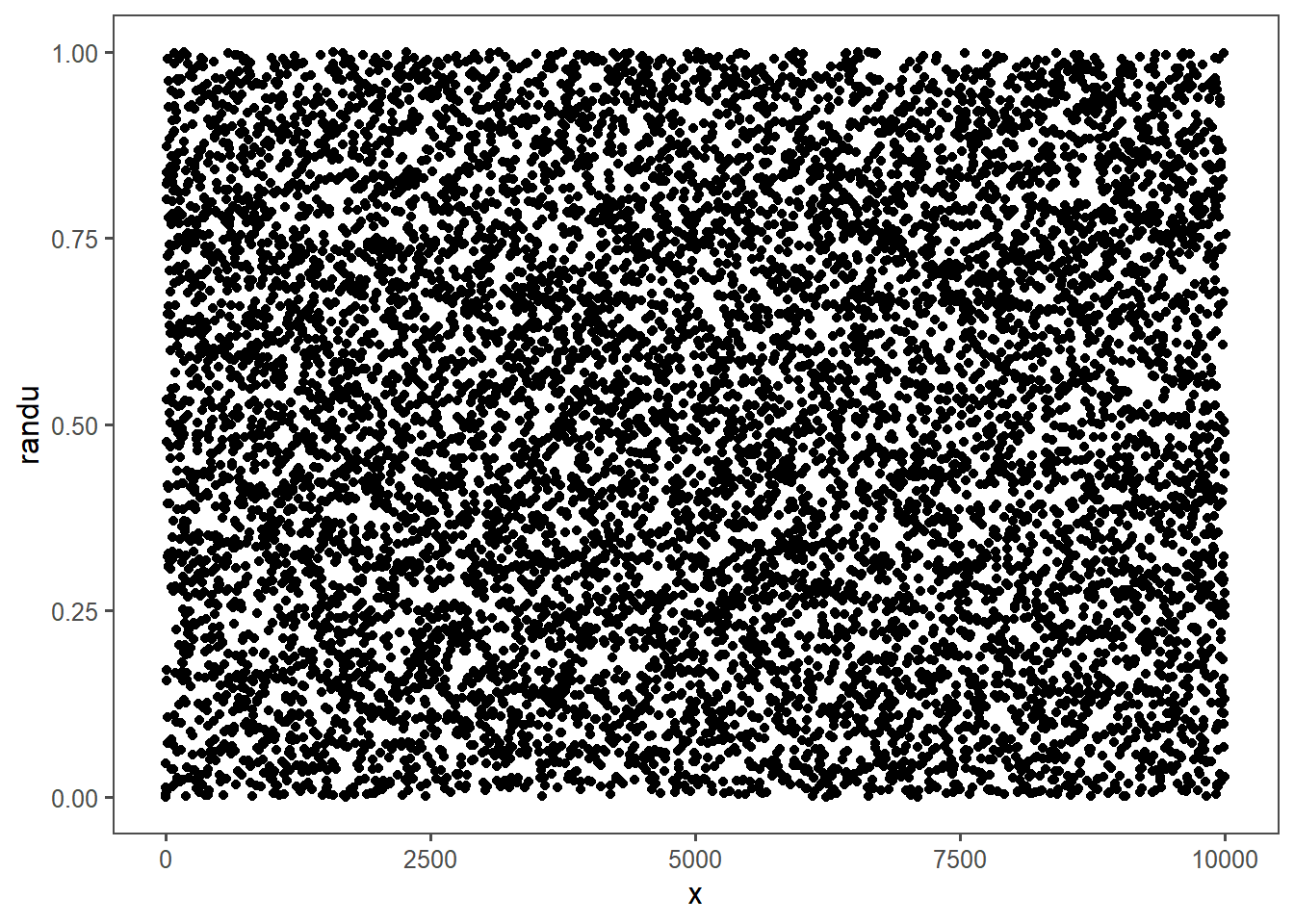
It takes a little time to get going, but once it’s going it looks like it’s bouncing all over the place. You can do a boxplot:
tibble(x = randu / (2^31)) %>%
  ggplot(aes(x = x)) +
  geom_boxplot()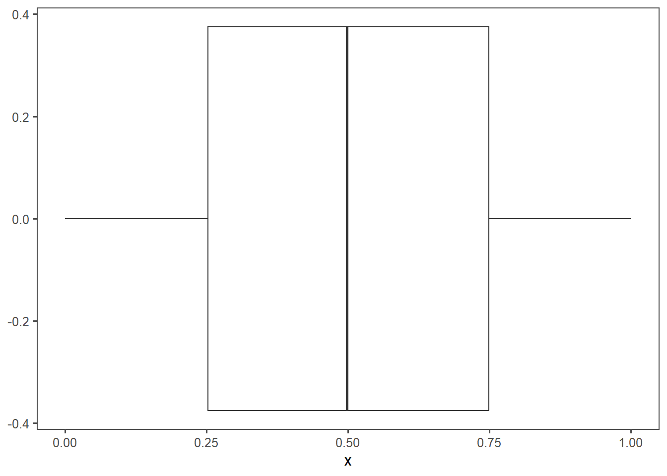
And the median is at 0.5, the quartiles are at 0.25 and 0.75, the whiskers go all the way to 0 and 1…
This algorithm stinks, and Knuth has described it as “truly horrible”.
I wasn’t great at number theory, but when I saw the algo something went off in my head. Maybe 8 perfect riffle shuffles as a highly related concept.
Anyway, what required 5-digit dollar hardware in the 1970s is now available in your web browser.
Behold RANDU in two dimensions, plotting against :
tibble(x = randu / (2^31)) %>%
  mutate(y = lag(x)) %>%
  ggplot(aes(x = x, y = y)) +
  geom_point()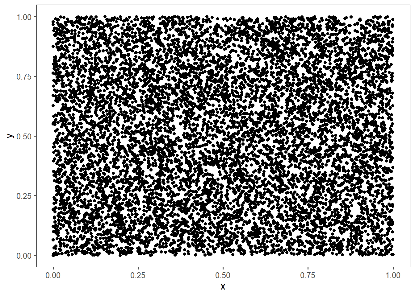
In 2d it still looks like it works. But in 3d:
tibble(x = randu / (2^31)) %>%
  mutate(y = lag(x)) %>%
  mutate(z = lag(y)) %>%
  plot_ly(x = ~x, y = ~y, z = ~z) %>%
add_markers(size = 0.1)Drag that around a bit. You’re looking for something like this.
I’m going to call this a special case of Schneier’s Law - anyone can construct a pseudorandom number generator that they can’t find a fault with. But with enough eyes any bug is shallow.