stationary biking with a raspberry pi

As well as lifting heavy weights, I cycle for my health. When it’s this cold, wet and windy I slot my bike into a stationary setup.

I’ll do some proper project photos and cross-link to a hardware hacking space, but I’ve connected a cheap bike computer (magnet + reed switch) to a Raspberry Pi, which has been told to log when this switch closes, once per revolution.

Github for the code for the bike

Anyway, I’m iterating this - test, refine, test.

Let’s load the last two rides and fix the current issues.

ride_2 = read_csv("https://github.com/jimr1603/stationary-bike/raw/main/2023-12-22%2020_18", col_names="time" ) %>% 
  mutate(time = as.POSIXct(time))
ride_1 = read_csv("https://github.com/jimr1603/stationary-bike/raw/main/2023-12-20%2017_01", col_names = "time") %>% 
  mutate(time = as.POSIXct(time))

circumference = 2.21 # wheel circumference, in meters.

ride_1 %>% 
  mutate(dt = as.numeric(time-lag(time))) %>% 
  mutate(dx = as_units(circumference, "m")) %>% 
  mutate(dt =as_units(dt, "seconds")) %>% 
  mutate(speed = dx/dt) %>% 
  mutate(speed = set_units(speed, "miles/hour")) %>% 
  ggplot(aes(x=time,y=speed)) + geom_point()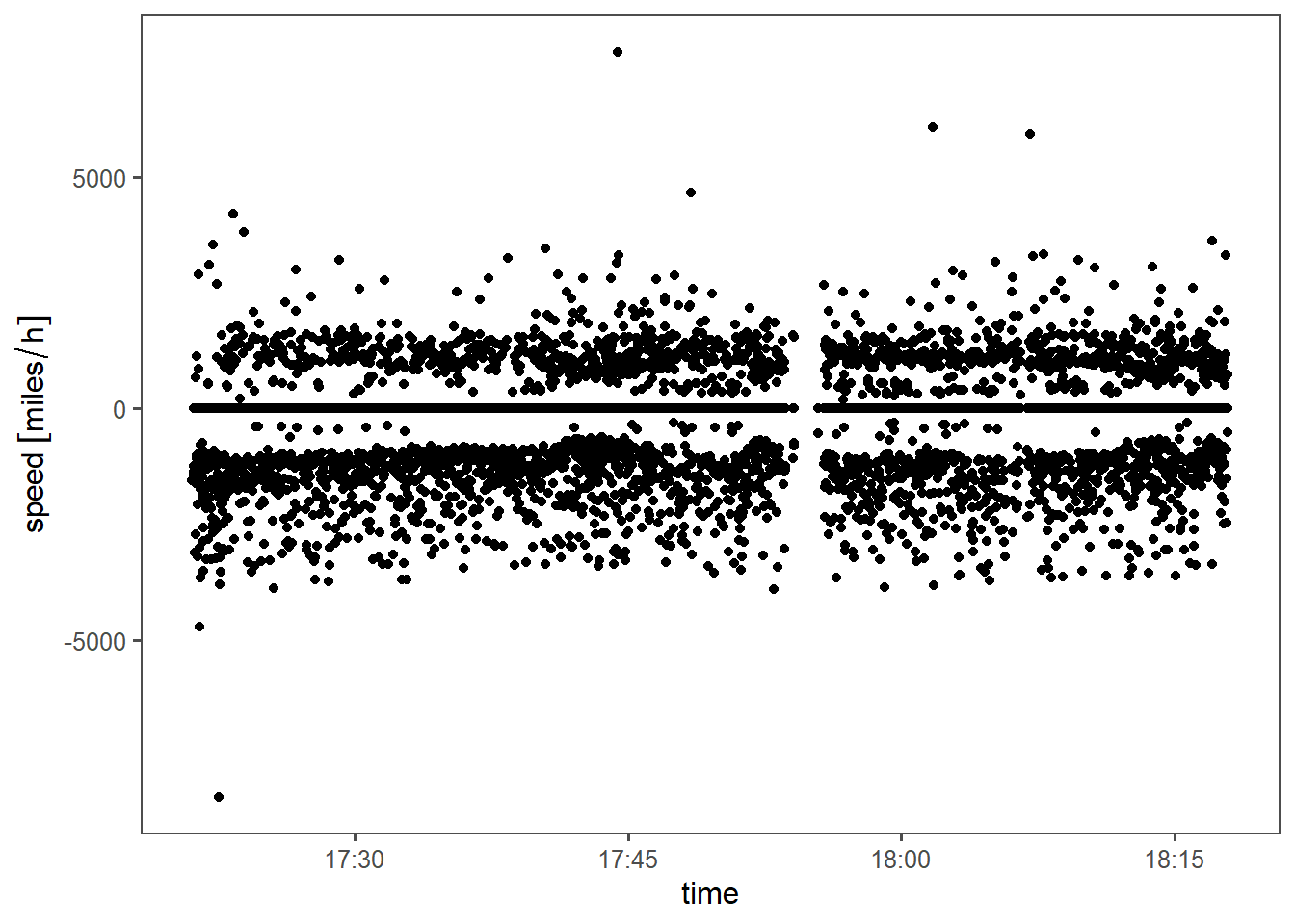

Negative speed?! Let’s remove that first.

ride_1 %>% 
  mutate(dt = as.numeric(time-lag(time))) %>% 
  mutate(dx = as_units(circumference, "m")) %>% 
  mutate(dt =as_units(dt, "seconds")) %>% 
  mutate(speed = dx/dt) %>% 
  filter(as.numeric(speed)>0) %>% 
  mutate(speed = set_units(speed, "miles/hour")) %>% 
  ggplot(aes(x=time,y=speed)) + geom_point()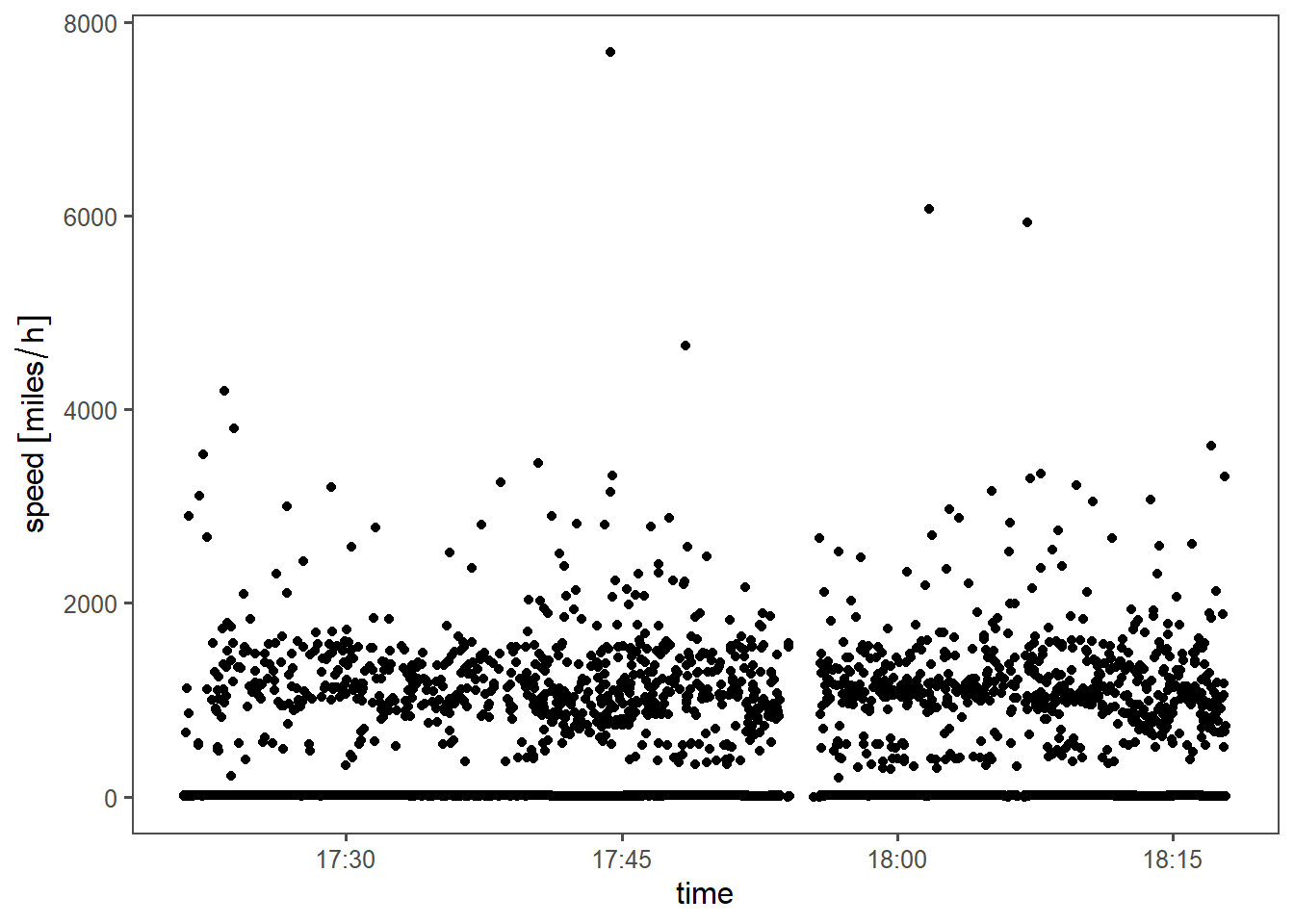

2000 miles per hour is so obviously bad, I’m going to try to zoom in. (Skipping several trial-and-error steps in where I choose my cutoff :D )

ride_1 %>% 
  mutate(dt = as.numeric(time-lag(time))) %>% 
  mutate(dx = as_units(circumference, "m")) %>% 
  mutate(dt =as_units(dt, "seconds")) %>% 
  mutate(speed = dx/dt) %>% 
  filter(as.numeric(speed)>0) %>% 
  mutate(speed = set_units(speed, "miles/hour")) %>% 
  filter(speed <= as_units(100, "miles/hour")) %>% 
  ggplot(aes(x=time,y=speed)) + geom_point()

So there’s a nice gap - under “100 miles/hour” the readings look sensible (except for negative time), and all readings over 100 miles per hour are sensor barf.

ride_1 %>% 
  mutate(dt = as.numeric(time-lag(time))) %>% 
  mutate(dx = as_units(circumference, "m")) %>% 
  mutate(dt =as_units(dt, "seconds")) %>% 
  mutate(speed = dx/dt) %>% 
  filter(as.numeric(speed)>0) %>% 
  mutate(speed = set_units(speed, "miles/hour")) %>% 
  filter(speed >= as_units(100, "miles/hour")) %>% 
  slice_min(speed)
## # A tibble: 1 × 4
##   time                    dt   dx     speed
##   <dttm>                 [s]  [m] [miles/h]
## 1 2023-12-20 17:56:49 0.0253 2.21      195.

It looks like the debounce time of 0.01 seconds is too small, I’ll try a debounce time of 0.03 for the next run.

If I manually throw out readings that are less than 0.03 secs from the last reading ¹ do the data look sensible?

ride_2 = read_csv("https://github.com/jimr1603/stationary-bike/raw/main/2023-12-22%2020_18", col_names="time" ) %>% 
  mutate(dt = time-lag(time)) %>%
  filter(dt > 0.03) %>% 
  mutate(dt = time-lag(time)) %>% 
  mutate(time = as.POSIXct(time))
ride_1 = read_csv("https://github.com/jimr1603/stationary-bike/raw/main/2023-12-20%2017_01", col_names = "time") %>% 
  mutate(dt = time-lag(time)) %>% 
  filter(dt > 0.03) %>% 
  mutate(dt = time-lag(time)) %>% 
  mutate(time = as.POSIXct(time))

ride_1 %>% 
  mutate(dt = as_units(dt, "seconds")) %>% 
  mutate(dx = as_units(circumference, "m")) %>% 
  mutate(speed = dx/dt) %>% 
  mutate(speed = set_units(speed, "miles/hour")) %>% 
  ggplot(aes(x=time,y=speed)) + geom_point()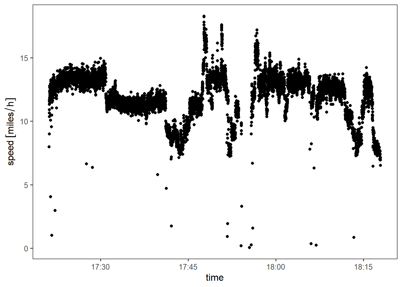

²

ride_2 %>% 
  mutate(dt = as_units(dt, "seconds")) %>% 
  mutate(dx = as_units(circumference, "m")) %>% 
  mutate(speed = dx/dt) %>% 
  mutate(speed = set_units(speed, "miles/hour")) %>% 
  ggplot(aes(x=time,y=speed)) + geom_point()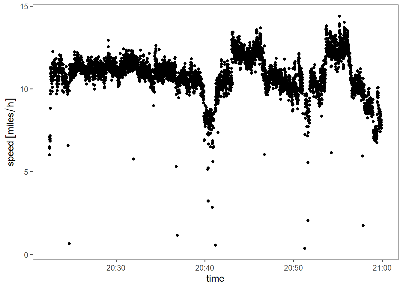

Even the ride I held back from the first analysis looks good :D

bind_rows(
  mutate(ride_1, id=1),
  mutate(ride_2, id=2)
) %>% 
  summarise(distance = circumference*n(), 
            duration = as.numeric(last(time)-first(time)),
            .by="id") %>% 
  mutate(distance = as_units(distance, "m"),
         duration = as_units(duration, "minutes")) %>% 
  mutate(avg_speed = set_units(distance/duration,"miles/hour")) %>% 
  knitr::kable()

id	distance	duration	avg_speed
1	17039.10 [m]	56.72568 [min]	11.19874 [miles/h]
2	10625.68 [m]	37.42866 [min]	10.58412 [miles/h]

Eyeballing recent rides, 10 or 11 miles per hour looks about right, give or take some hills. I’ll keep the wheel circumference of 2.21 m, push a debounce on the switch of 0.03 seconds, and have another ride.