Sometimes I see a Riddler Classic that makes me just want to go attack it with Monte Carlo analysis.
Let’s make a die and roll it 6 times, recording the outcome:
die <- 1:6

faces <- sample(seq_along(die), length(die), replace=T) # referring to the length of the die vector will help us if we do the extra credit

die <- die[faces]

die
## [1] 3 2 1 5 1 3
That’s 1 iteration. Loops will be necessary since I need the 2nd die to produce the 3rd die, so R’s clever vectorisation won’t help.
I’d like to track a ‘score’ - how far we are from the target of all faces equal. Let’s say the score is the number of distinct numbers still on the die, and the target is a score of 1.
update_die <- function(die){

  faces <- sample(seq_along(die), length(die), replace=T) # referring to the length of the die vector will help us if we do the extra credit

  die[faces]
}
update_score <- function(die){
  unique(die) %>%
  length()
}

die <- 1:6
score <- update_score(die)

while(last(score) >1){
  die <- update_die(die)

  score <- c(score, update_score(die))
}
Anything we can do 1ce, we can do many times.
simulate_1_game <- function(index, size_of_die){
  die <- seq_len(size_of_die)
  score <- update_score(die)

  while(last(score) >1){
    die <- update_die(die)

    score <- c(score, update_score(die))
  }

  games <- seq_along(score)
  tibble(index=index, score=score, game=games)
}

monte_carlo_d6 <- map_dfr(seq_len(1e4), ~simulate_1_game(.x,6))
monte_carlo_d6 %>%
ggplot(aes(x=game, after_stat(density))) + geom_freqpoly(binwidth=1) + facet_wrap(~score, ncol=1, scales = "free_y") +
theme + scale_y_continuous(labels=scales::percent)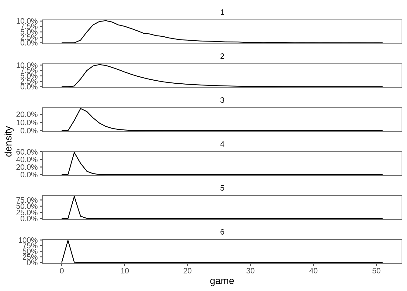
monte_carlo_d6 %>%
  tabyl(game, score) %>%
  pivot_longer(-game, names_to = "score") %>%

  ggplot(aes(x=game,y=value,fill=score)) + geom_area() + theme + ggthemes::scale_fill_few()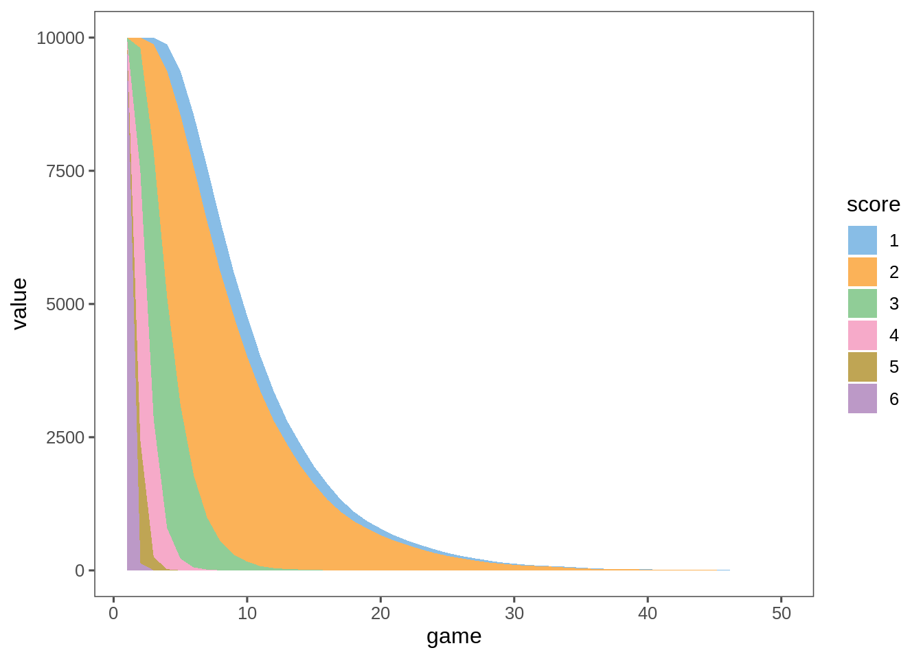
monte_carlo_d6 %>%
  group_by(index) %>%
  summarise(games_until_win = max(game)) %>%
  ggplot(aes(x=games_until_win, after_stat(density)))  + geom_freqpoly(binwidth = 1) +
    theme + scale_y_continuous(labels=scales::percent)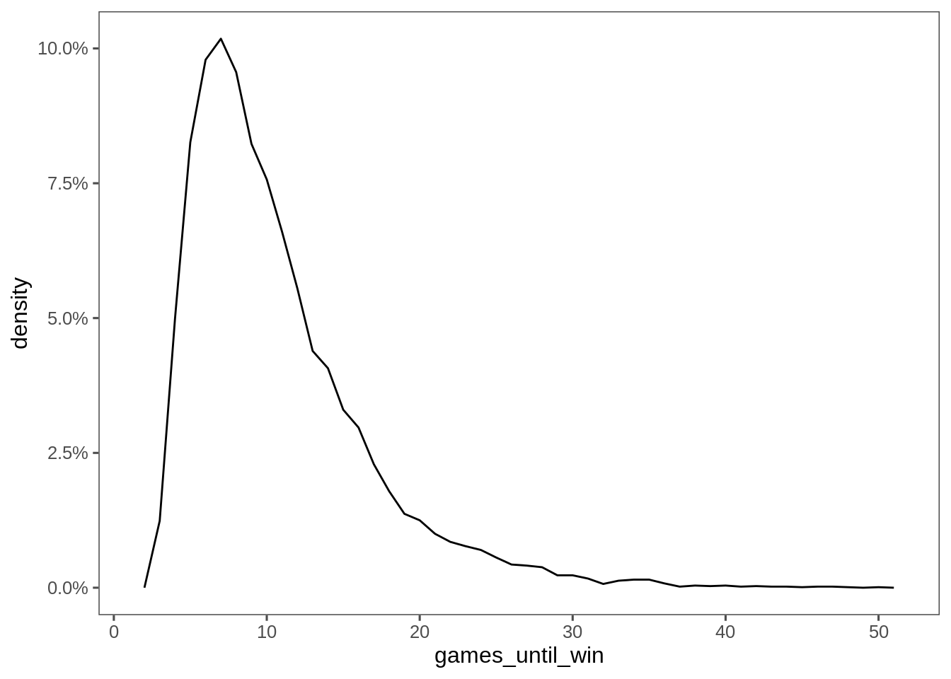
monte_carlo_d6 %>%
  group_by(index) %>%
  summarise(games_until_win = max(game)) %>%
  tabyl(games_until_win) %>%
  mutate(percent = scales::percent(percent)) %>%
knitr::kable()| games_until_win | n | percent |
|---|---|---|
| 3 | 124 | 1.2% |
| 4 | 499 | 5.0% |
| 5 | 826 | 8.3% |
| 6 | 979 | 9.8% |
| 7 | 1018 | 10.2% |
| 8 | 956 | 9.6% |
| 9 | 823 | 8.2% |
| 10 | 757 | 7.6% |
| 11 | 660 | 6.6% |
| 12 | 555 | 5.6% |
| 13 | 439 | 4.4% |
| 14 | 407 | 4.1% |
| 15 | 330 | 3.3% |
| 16 | 297 | 3.0% |
| 17 | 229 | 2.3% |
| 18 | 179 | 1.8% |
| 19 | 137 | 1.4% |
| 20 | 125 | 1.2% |
| 21 | 100 | 1.0% |
| 22 | 85 | 0.8% |
| 23 | 77 | 0.8% |
| 24 | 70 | 0.7% |
| 25 | 56 | 0.6% |
| 26 | 43 | 0.4% |
| 27 | 41 | 0.4% |
| 28 | 38 | 0.4% |
| 29 | 23 | 0.2% |
| 30 | 23 | 0.2% |
| 31 | 17 | 0.2% |
| 32 | 7 | 0.1% |
| 33 | 13 | 0.1% |
| 34 | 15 | 0.2% |
| 35 | 15 | 0.2% |
| 36 | 8 | 0.1% |
| 37 | 2 | 0.0% |
| 38 | 4 | 0.0% |
| 39 | 3 | 0.0% |
| 40 | 4 | 0.0% |
| 41 | 2 | 0.0% |
| 42 | 3 | 0.0% |
| 43 | 2 | 0.0% |
| 44 | 2 | 0.0% |
| 45 | 1 | 0.0% |
| 46 | 2 | 0.0% |
| 47 | 2 | 0.0% |
| 48 | 1 | 0.0% |
| 50 | 1 | 0.0% |
Other dice
We’d like to keep track of the size of our dice, tweak the simulate function. Just going to track average games until win to save on memory.
rm(monte_carlo_d6)
estimate_victory <- function(size_of_die){
original_die <- seq_len(size_of_die)
die <- original_die
dice_pool <- sample(original_die, 1000*size_of_die, replace=T)
play_1_game <- function(...){
n=0L
score <- 10
while(last(score) > 1){
if(length(dice_pool) < size_of_die){
dice_pool <<- sample(original_die, 100*size_of_die, replace=T)
}
n <- n+1L
die <- die[dice_pool[original_die]]
dice_pool <<- dice_pool[-original_die] #Pop 1:n from the dice pool.
score <- c(score, update_score(die))
}
return(n)
}
map_int(1:1000, play_1_game) %>%
mean()
}
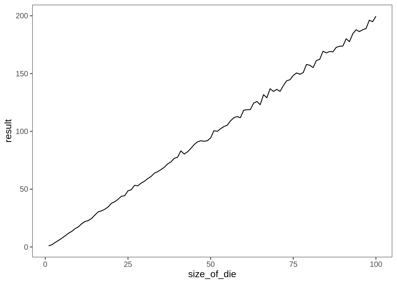
results <- future_map_dbl(1:100, estimate_victory)Looks pretty much linear, and might end up more linear if I gave it more simulation time.
tibble(size_of_die = 1:100, result=results) %>%
  ggplot(aes(x=size_of_die,y=result)) + theme + geom_line()