Odin
Package Odin has gone live on CRAN with version 1. It makes some stuff with deSolve a little easier: - Defining a set of ODEs looks a bit easier - it’s easier to change parameters - it can write its own C code for when you’ve got a massive set of ODEs and the efficiency helps.
Also, it’s a great punny name.
Lorentz’s Butterfly
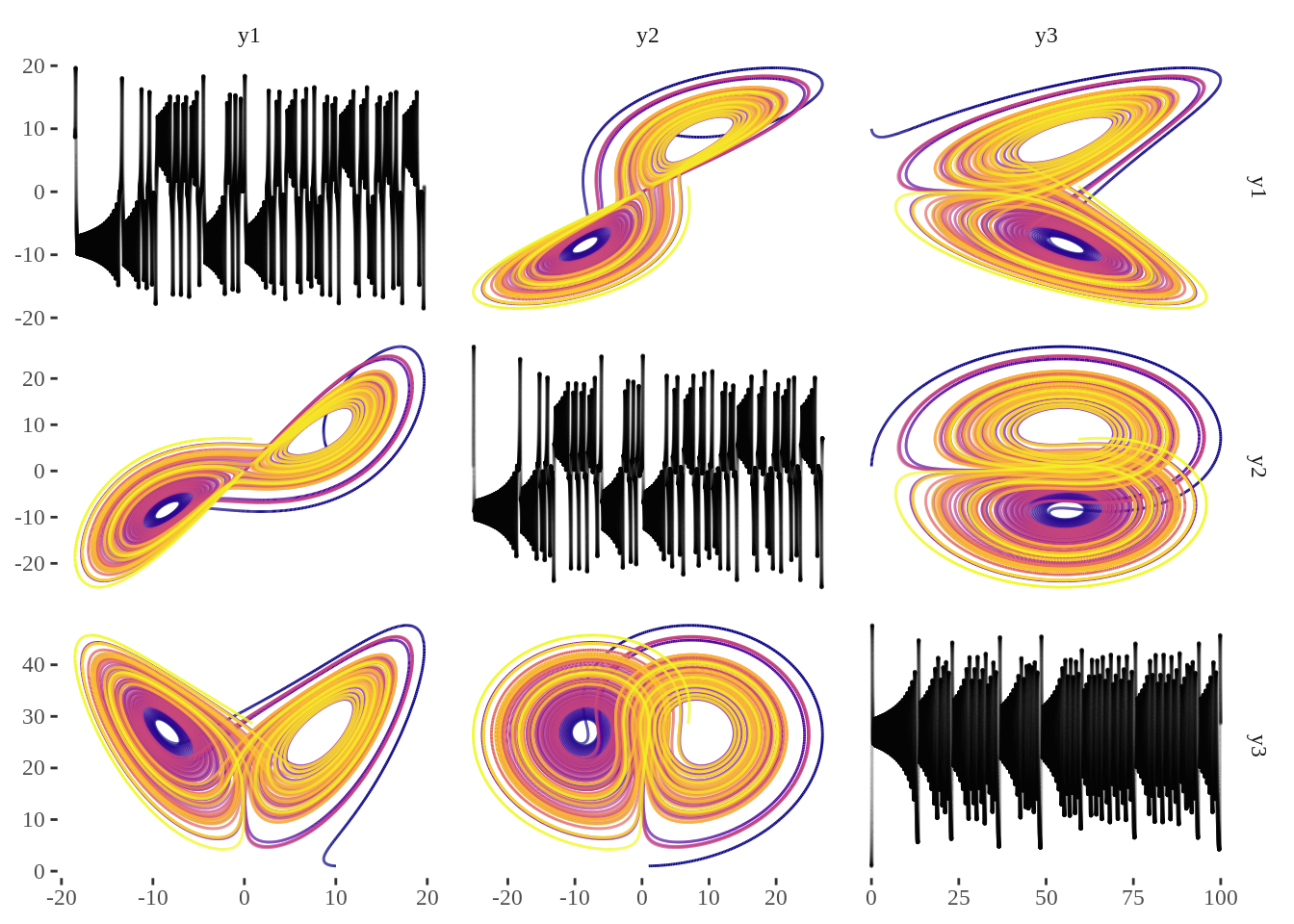
Lorentz was trying to study a very simplified weather model with early computers. It’s easily described in 3 dimensions with respect to time - Link to his paper. At least skim it for the pictures, this is 1960’s fractal art! The 3 dimensions don’t seem to have simple interpretations once they’ve gone into this form.
It’s incredibly sensitive to initial conditions, he had problems trying to resume a simulation from a printout that only had 3 decimals, but the computer held more in memory.
library(odin)
library(GGally)
lorentz <- odin({
deriv(y1) <- sigma * (y2 - y1)
deriv(y2) <- R * y1 - y2 - y1 * y3
deriv(y3) <- -b * y3 + y1 * y2
initial(y1) <- start_y_1
initial(y2) <- start_y_2
initial(y3) <- start_y_3
start_y_1 <- user(10)
start_y_2 <- user(1)
start_y_3 <- user(1)
## These are the classical parameters:
sigma <- 10
R <- 28
b <- 8 / 3
})
## gcc -std=gnu99 -I"/usr/share/R/include" -DNDEBUG -fpic -g -O2 -fdebug-prefix-map=/build/r-base-el7SHG/r-base-3.5.2=. -fstack-protector-strong -Wformat -Werror=format-security -Wdate-time -D_FORTIFY_SOURCE=2 -g -c odin_a305fa58.c -o odin_a305fa58.o
## gcc -std=gnu99 -shared -L/usr/lib/R/lib -Wl,-Bsymbolic-functions -Wl,-z,relro -o odin_a305fa58.so odin_a305fa58.o -L/usr/lib/R/lib -lR
model <- lorentz()
tt <- seq(0, 100, by=1e-3)
model_result <- model$run(tt,method="lsode" ) %>%
as_tibble() %>%
mutate_all(as.numeric)
path <- function(data, mapping){
ggplot(data=data, mapping=mapping) +
geom_path( aes(colour=t)) +
scale_color_viridis_c(option = "C") +
ggthemes::theme_tufte()
}
self <- function(data, mapping){
ggplot(data=data, mapping=mapping) + geom_point(aes(y=t), size=0.1,alpha=0.1) + coord_flip()
}
model_result %>%
ggpairs(columns =c("y1","y2","y3"),
upper=list(continuous=path),
diag=list(continuous=self),
lower=list(continuous=path)) + ggthemes::theme_tufte()
It has 3 spatial dimensions, and 1 dimension of time, so let’s throw it at more stuff.
model_result %>%
mutate(s=round(t,0)) %>%
plot_ly(x=~y1,y=~y2,z=~y3, color=~t) %>%
add_paths()And if a butterfly flaps its wings
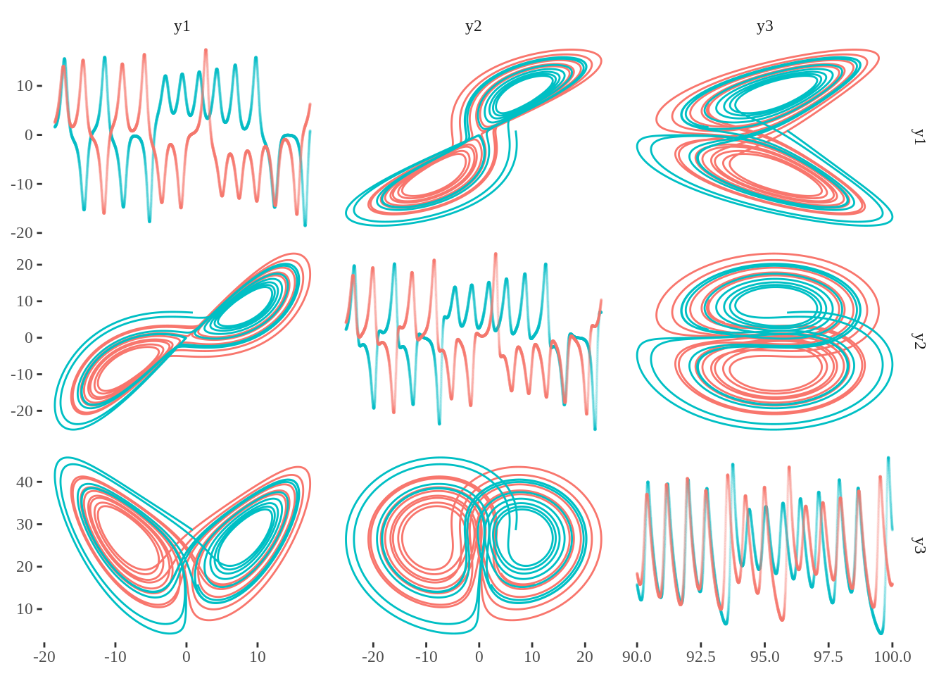
If I give the system a slight nudge in its starting conditions, then it ends up in a totally different bit of its phase space.
butterfly <- 1e-6
interfering_butterfly <- lorentz(start_y_1 = 10+butterfly, start_y_2 = 1+butterfly, start_y_3 = 1+butterfly)
interfering_butterfly <- interfering_butterfly$run(tt)%>%
as_tibble() %>%
mutate_all(as.numeric) %>%
mutate(model="butterfly")
model_result <- mutate(model_result, model="original")
path <- function(data, mapping){
ggplot(data=data, mapping=mapping) +
geom_path( aes(colour=model)) +
ggthemes::theme_tufte()
}
self <- function(data, mapping){
ggplot(data=data, mapping=mapping) + geom_point(aes(y=t, colour=model), size=0.1,alpha=0.1) + coord_flip()
}
bind_rows(model_result, interfering_butterfly) %>%
filter(between(t,90, 100)) %>%
ggpairs(columns =c("y1","y2","y3"),
upper=list(continuous=path),
diag=list(continuous=self),
lower=list(continuous=path)) + ggthemes::theme_tufte()
I think the original story involves a printout to 3 decimals, so it’s nice to see them disagree quickly for a difference in 6 decimals.
bind_rows(model_result, interfering_butterfly) %>%
plot_ly(x=~y1,y=~y2,z=~y3, split=~model) %>%
add_paths()