I have a folder of data waiting to be played with. The playing with is the interesting part. Most of the inertia is over the cleaning the data part.
One of these datasets is Stats19, provided by DfT under the OGL. There’s now a package for easy loading of a cleaned dataset: stats19. Note the comment about how prior to its release they estimate about 80% of time spent working with these data was on doing similar cleaning that everyone else was doing!
For now, I’m going to work with 2017 data. A later post might look at trends.
crashes <- get_stats19(year = 2017, type = "Accidents", ask = FALSE)
casualties <- get_stats19(year = 2017, type = "Casualties", ask = FALSE)
vehicles <- get_stats19(year = 2017, type = "Vehicles", ask = FALSE)
Straight away, 170993 casualties in 2017. Splitting these out:
casualties %>%
  group_by(casualty_severity) %>%
  summarise(n=n()) %>%
knitr::kable()| casualty_severity | n |
|---|---|
| Fatal | 1793 |
| Serious | 24831 |
| Slight | 144369 |
With 3 classes of casualty, a facet wrap makes sense.
casualties %>%
filter(age_of_casualty >= 0) %>% #Keep only the ones whose age is known.
ggplot(aes(x=age_of_casualty)) + geom_density() + facet_wrap(~casualty_severity) + ggthemes::theme_few()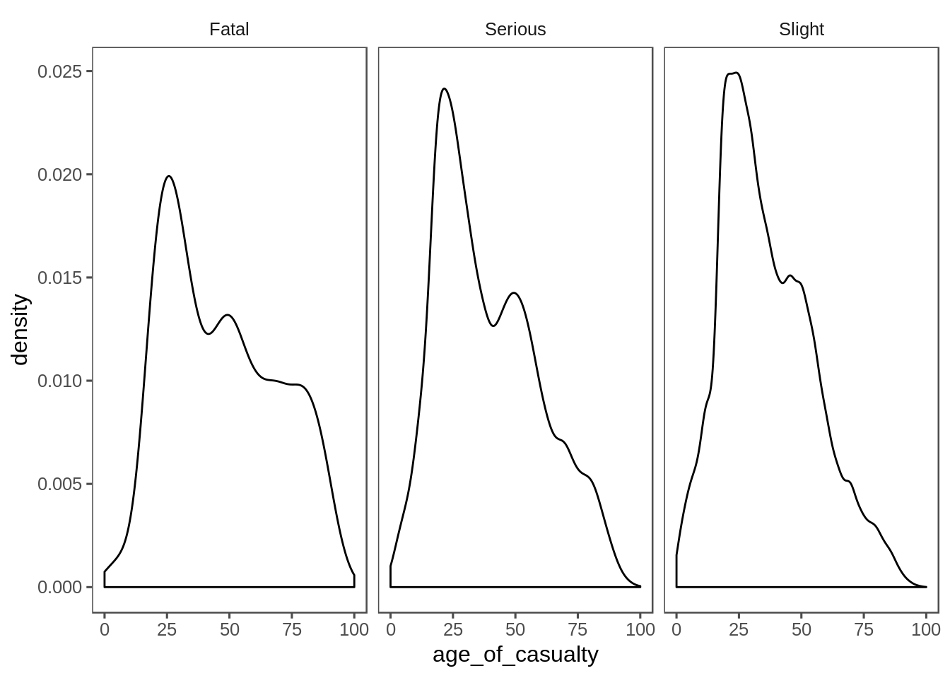 The differences by sex are interesting:
casualties %>%
filter(age_of_casualty >= 0) %>%
filter(sex_of_casualty %in% c("Male", "Female")) %>%
ggplot(aes(x=age_of_casualty, colour=sex_of_casualty)) + geom_density() + facet_grid(~casualty_severity) + ggthemes::theme_few() + ggthemes::scale_colour_few()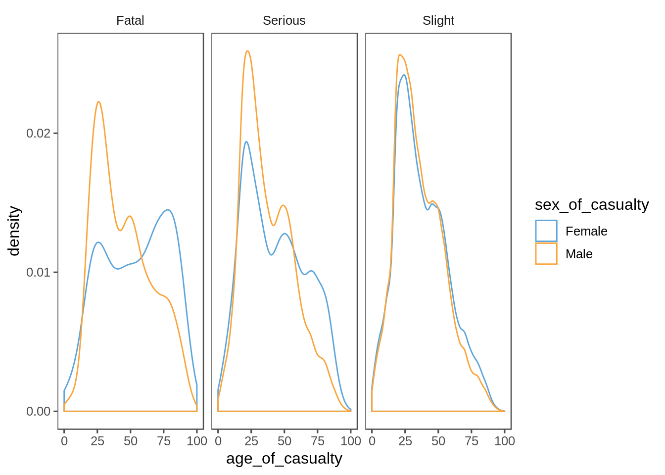 (Yeah, I’m being lazy and keeping the snake_case names in the graphs.)
Where are Agricultural vehicles crashing?
ids <- vehicles %>%
  filter(vehicle_type == "Agricultural vehicle")  %>%
  pull(accident_index)

agri_crashes <- crashes %>%
    filter(accident_index %in% ids) %>%
    format_sf()

agri_crashes %>%
    select(id=accident_index ) %>%
    aggregate(by=police_boundaries, FUN=length) %>%
    plot()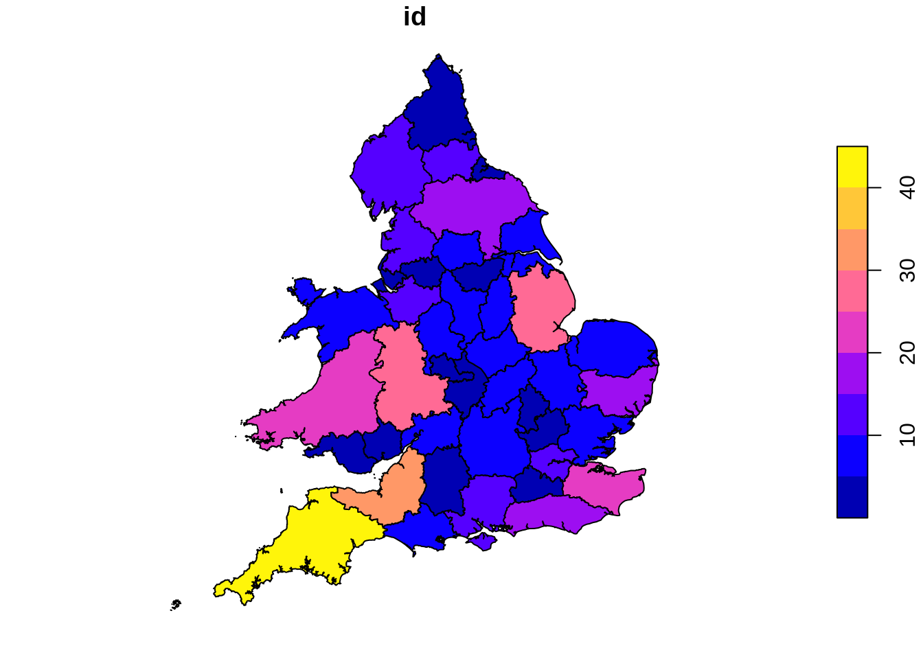
The areas commonly associated with farming. So far, this makes sense.
Manually rooting around the data, I found a crash where a mobility scooter had a passenger. (Thankfully not fatal.) So I’m now going to poke the data for incidents involving a mobility scooter, and no other vehicle. Maybe pedestrians.
scooter_ids <- vehicles %>%
  filter(vehicle_type == "Mobility scooter") %>%
  pull(accident_index)

scooter_and_another_vehicle <- vehicles %>%
  filter(accident_index %in% scooter_ids) %>%
  filter(vehicle_type != "Mobility scooter") %>%
  pull(accident_index)

ids <- setdiff(scooter_ids, scooter_and_another_vehicle)

scooter_only <- crashes %>%
  filter(accident_index %in% ids)

nrow(scooter_only)
## [1] 65
65 crashes involved a mobility scooter and no other vehicle.
casualties %>%
  filter(accident_index %in% ids) %>%
  group_by(casualty_severity) %>%
  summarise(n=n()) %>%
knitr::kable()| casualty_severity | n |
|---|---|
| Fatal | 1 |
| Serious | 17 |
| Slight | 51 |
casualties %>%
  filter(accident_index %in% ids) %>%
  group_by(casualty_class) %>%
  summarise(n=n()) %>%
knitr::kable()| casualty_class | n |
|---|---|
| Driver or rider | 14 |
| Pedestrian | 55 |
But 69 casualties, including 1 fatal. Most of the injuries were received by pedestrians.
crashes %>%
  filter(accident_index %in% ids) %>%
  format_sf() %>%
  select(id = accident_index) %>%
  aggregate(by=police_boundaries, FUN=length) %>%
  plot()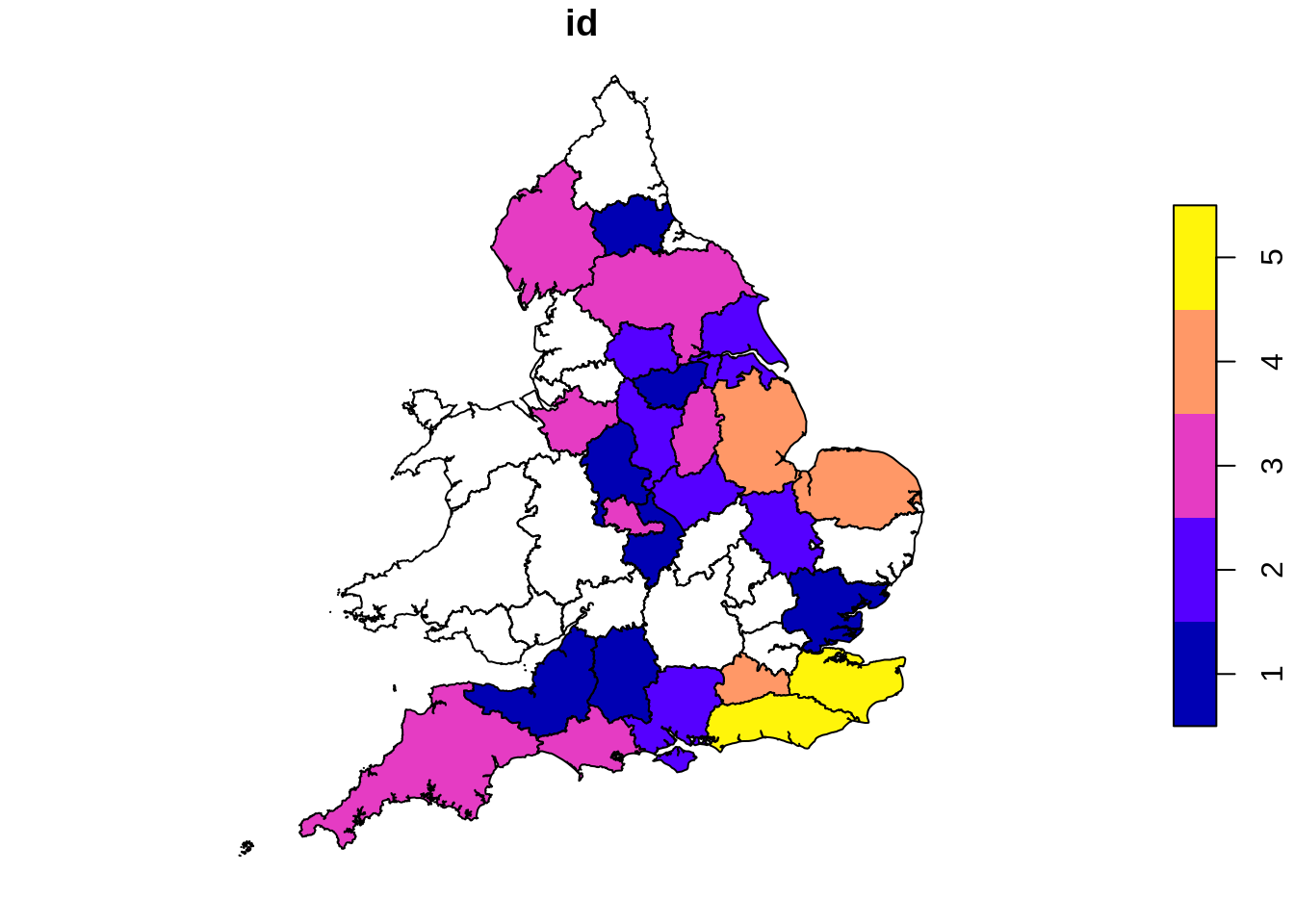
When your binning ends up with unique values, you know that you’re looking at a very rare event. Some patterns might emerge with more years of data, but I wouldn’t bet on it.
Cycling
casualties %>%
  filter(casualty_type == "Cyclist") %>%
  group_by(casualty_severity) %>%
  summarise(n=n()) %>%
  mutate(proportion=n/sum(n)) %>%
knitr::kable()| casualty_severity | n | proportion |
|---|---|---|
| Fatal | 101 | 0.0055128 |
| Serious | 3698 | 0.2018449 |
| Slight | 14522 | 0.7926423 |
casualties %>%
  filter(casualty_type != "Cyclist") %>%
  group_by(casualty_severity) %>%
  summarise(n=n()) %>%
  mutate(proportion=n/sum(n)) %>%
knitr::kable()| casualty_severity | n | proportion |
|---|---|---|
| Fatal | 1692 | 0.0110828 |
| Serious | 21132 | 0.1384171 |
| Slight | 129845 | 0.8505001 |
So, how safe is cycling? Well nationally, if you’re in a crash that the police show up to, you’re less likely to be dead, but more likely to be severely injured as a cyclist than a non-cyclist.
(What about the crashes the police don’t turn up to? We don’t know! Can’t get Official Stats on events that aren’t recorded.)
What about my home West Yorkshire?
wy_boundary <-  police_boundaries[police_boundaries$pfa16nm == "West Yorkshire", ]

wy_crashes <- crashes %>%
  format_sf()
wy_crashes <- wy_crashes[wy_boundary, ]

casualties %>%
  filter(accident_index %in% wy_crashes$accident_index) %>%
  filter(casualty_type == "Cyclist") %>%
  group_by(casualty_severity) %>%
  summarise(n=n()) %>%
  mutate(proportion=n/sum(n)) %>%
knitr::kable()| casualty_severity | n | proportion |
|---|---|---|
| Serious | 121 | 0.2122807 |
| Slight | 449 | 0.7877193 |
casualties %>%
  filter(accident_index %in% wy_crashes$accident_index) %>%
  filter(casualty_type != "Cyclist") %>%
  group_by(casualty_severity) %>%
  summarise(n=n()) %>%
  mutate(proportion=n/sum(n)) %>%
knitr::kable()| casualty_severity | n | proportion |
|---|---|---|
| Fatal | 42 | 0.0080245 |
| Serious | 688 | 0.1314482 |
| Slight | 4504 | 0.8605273 |
I could do some fancy statistical tests, but W Yorks looks fairly similar to the national average for these stats. There’d be about 3 bike fatalities if it were exact, but 0 is close to 3, for these purposes.
Male drivers more dangerous?
A truism I was told for why all else equal male car insurance used to be higher than that for female, was that men crashed less often than women, but the crashes tended to be more expensive. This is not the right dataset to investigate that fully. But we can look at outcomes when:
- the police showed up.
- there was at least one car involved.
- the sex of all drivers was recorded.
Another caveat is that we don’t know who was “at fault”, so we don’t know which way the insurance will have settled, which is what the just-so claim at the start was about.
male_driving <- vehicles %>%
  filter(sex_of_driver == "Male", vehicle_type == "Car") %>%
  pull(accident_index)

unknown_other <- vehicles %>% #Filter out accident IDs where there's someone of unknown sex driving a car.
  filter(accident_index %in% male_driving) %>%
  filter(vehicle_type == "Car", sex_of_driver == "Not known") %>%
  pull(accident_index)

male_driving <- setdiff(male_driving, unknown_other)

female_driving <- vehicles %>%
  filter(sex_of_driver == "Female", vehicle_type == "Car") %>%
  pull(accident_index)


unknown_other <- vehicles %>% #Filter out accident IDs where there's someone of unknown sex driving a car.
  filter(accident_index %in% female_driving) %>%
  filter(vehicle_type == "Car", sex_of_driver == "Not known") %>%
  pull(accident_index)

female_driving <- setdiff(female_driving, unknown_other)
Some summary stats are available in the crashes table:
male_crash <- crashes %>%
  filter(accident_index %in% male_driving) %>%
  select(accident_severity, number_of_casualties) %>%
  mutate(sex = "Male")

female_crash <- crashes %>%
  filter(accident_index %in% female_driving) %>%
  select(accident_severity, number_of_casualties) %>%
  mutate(sex = "Female")

##In crashes where there was a male driver and a female driver, we've double counted.

gendered_crashes <- bind_rows(male_crash, female_crash)

gendered_crashes %>%
  group_by(sex, accident_severity) %>%
  summarise(n=n()) %>%
  ggplot(aes(x=accident_severity, y=n, colour=sex)) + geom_point() + ggthemes::theme_few() + ggthemes::scale_colour_few()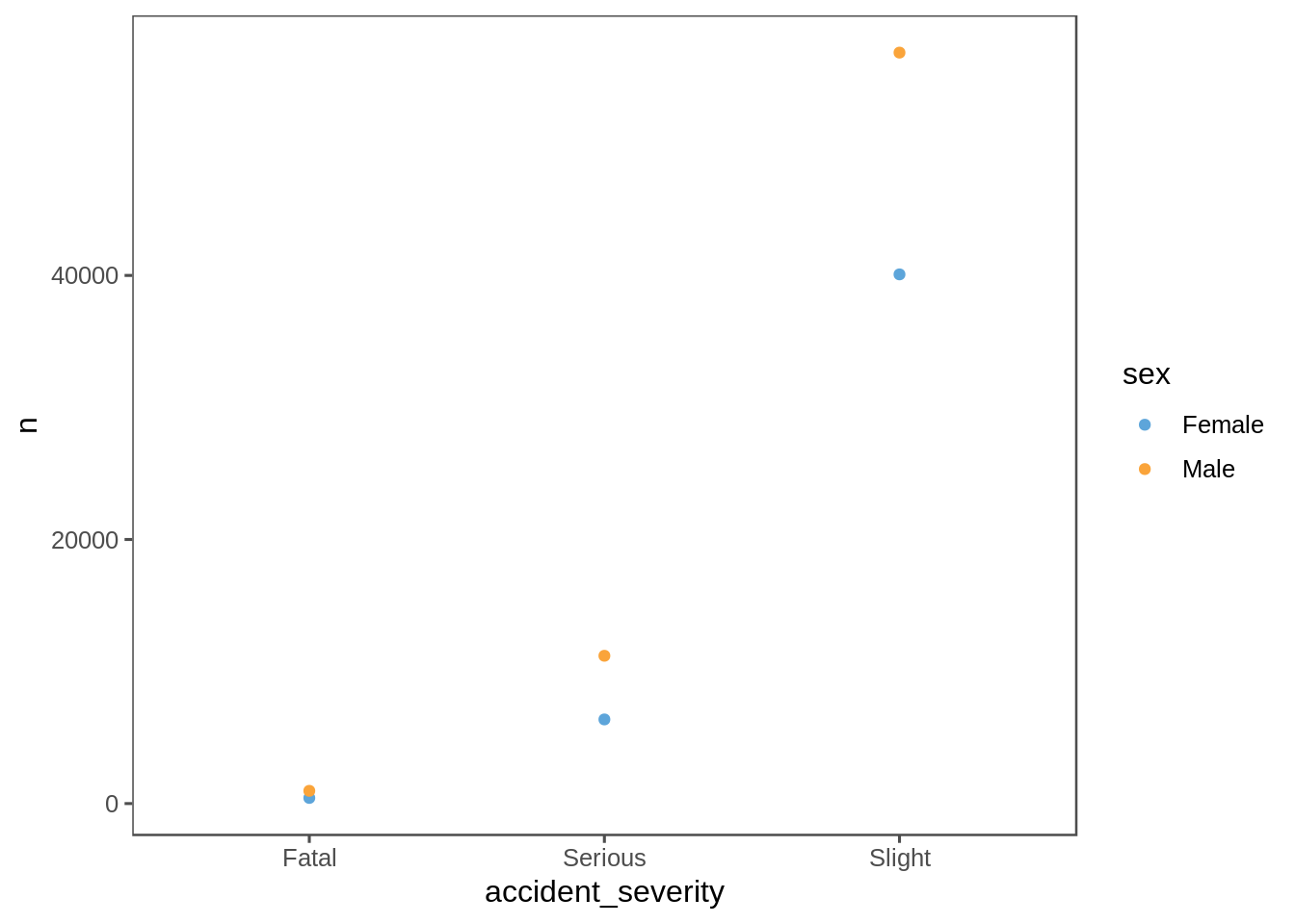
The just-so story at the beginning of this section looks shaky - men get into more crashes where the police are involved.
gendered_crashes %>%
  group_by(sex, number_of_casualties) %>%
  summarise(n=n()) %>%
  ggplot(aes(x=number_of_casualties, y=n, colour=sex)) + geom_point() + ggthemes::theme_few() + ggthemes::scale_colour_few()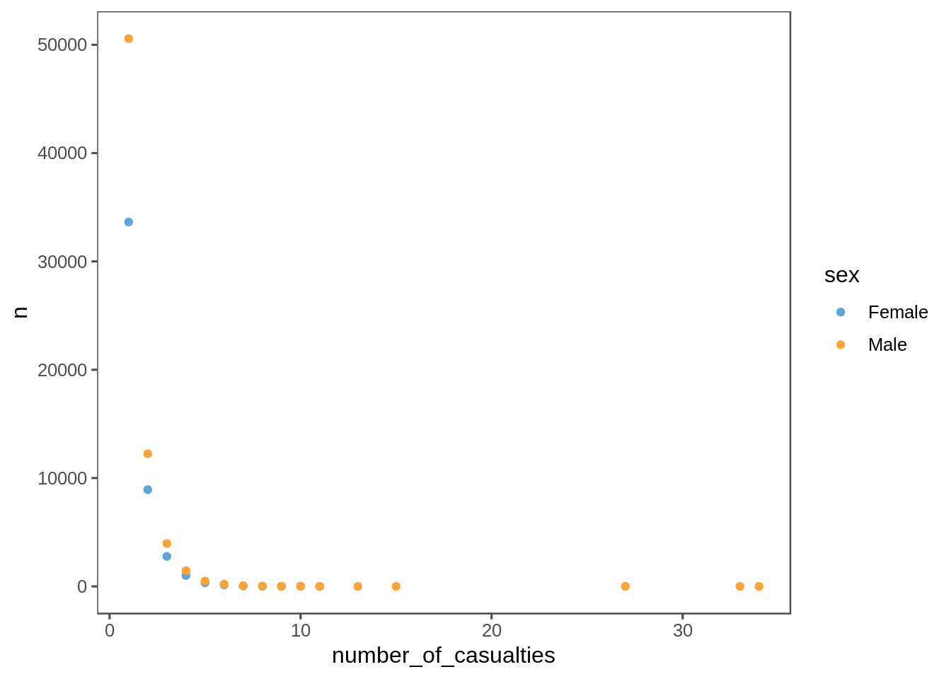
Has Ziph’s Law cropped up in yet another place?
I was thinking of digging into the coarser casualty data, but it’s clear that as far as this dataset is concerned watch out for men driving cars.
Future ideas:
I want to play with leaflet. And since the tiles default to OSM, there might be some fun stuff with investigating if it’s safer to be a cyclist where there’s various types of infrastructure. This dataset doesn’t have a lot of that, but the public have been quite good at mapping cycle lanes on OSM.
I’ve not touched on the fact that these data go back to 1979. If messing around with OSM gets any info on when various infrastructure changed, can I see a change in the stats?