Motivation
As I just had another birthday with a ‘0’ at the end, I’m thinking about how long I have left.And it relates to other forecasts I could make, like will I ever pay off my student loans? The ONS publish national life tables under the OGL, so we have the data, and the permission to use it. And straight away I can see that the average UK 30-year old male has about 50 years left.
But I want more than that.I want a probability distribution. I want to know my chance of living to certain events, like Halley’s Comet, or retirement, or the day my student loans get written off. (Obviously, dying before my loans are paid off means that I never pay them off!) ONS have given me the cutoff where it’s equally likely I’ll be dead or alive, but what if I’m being risk-averse and want to consider \(p<50%\)? Values are given by year, what if I wanted month or day? (This would be a terrible idea, there’s already enough uncertainty in the numbers.)
Caveats
These tables are produced for population-level modelling. Probability is happiest when you repeat a test many, many times, like when you have a population of 70 million people. I am one person, and the universe doesn’t want to let me live my life many, many times as an experiment.
The following is mostly intended as a demonstration of how I like to think about probability despite always getting combinatorics wrong. I like monte-carlo methods, particularly where a number is wanted to a certain precision, rather than an exact formula.
Modelling
With this sort of model/program, I like to break it down into stages:
- Work out the process for one person.
- Work out the subprocesses needed to handle one person.
- Model one person once.
- Model one person many times.
- Model many people many times.
I plan to get to (4) in this post, and eventually write a R htmlwidget so that any visitor can get a personalised memento mori.
mortality_tables <- read_csv(here("static","data","Open Government Licence","uk mortality 14-16.csv"))Here’s where a decade of playing tabletop RPGs comes in handy. In a given test, I survive if I roll a die that can take values between 0 and 1 and roll above the probability of death. (I pass my con check?) I don’t have to worry about my survival rates between 0 and 30, because I’ve already done those. I’ll do a longer post later on conditional probability, but for now consider the absurdity of a model that says I have -1 years to live! So for now I might as well just keep the probabilities for years 30+:
mortality_vector <- mortality_tables %>%
  filter(Age>=30) %>%
  select(-Females) #A negative select keeps everything but that column

datatable(mortality_vector)
Learning the R way of doing things is an ongoing process, so what I did first was try to start at year 30, roll a number, see if I survive, if so move onto the next number, if not then report the year of death. This was easy when mortality_vector was an actual vector, but it’s easy to see a better method with the pipe:
one_run <- mortality_vector %>%
  mutate(rolled_dice = runif(nrow(mortality_vector))) %>%
  filter(rolled_dice < Males) %>%
  top_n(-1, Age)

datatable(one_run)
So, for those keeping up, I’ve reached (3) in my list of things to do. Now I just need to generate many, many James’ and watch them die. There are a few ways to do this.
- Take the above process, wrap it into a function, tell it to repeat \(n\) times and output a bunch of values I can put into a histogram. The problem with this is that every loop we’ll call
runif. R is a lot happier calling generating a lot of random numbers once, rather than doing a few random numbers a lot of times.
So let’s add a massive number of columns to mortality_vector and then look at how we turn that into values. For now let’s call the number of repetitions nreps, and give it some value.
nreps <- 10
f <- function(x){return(x)} #I don't currently have an elegant way to pass this to detect_index

tibble_method <- function(nreps) {
results <- matrix(runif(nreps*nrow(mortality_vector)), ncol=nreps) %>%
  as_tibble() %>%
  mutate_all(funs(.<mortality_vector$Males)) %>%
  map(detect_index, f)

  return(results)
}
But then I want to get the least element where a death happens in each column, and extract the age. Time to learn Purr, the iteration library in the Tidyverse.
age_at_death <- function(age_now, sex) {
  return_value <- mortality_tables %>%
    filter(Age >=age_now) %>%
    select(-Females) %>% #TODO: make it so it actually selects appropriate sex, not just "Males"
    mutate(rolled_dice = runif(nrow(mortality_vector))) %>%
    filter(rolled_dice < Males) %>%
    top_n(-1, Age) %>%
    pull(Age)
  if(length(return_value)==0){return_value=101} #handle case where live past 100
  return(list("dead"=return_value))
}

params = list( "age_now" = c(30), "sex"=c("Male"))
Comparison
MonteCarlo package generalises nicely. Especially if you’re running over a wide parameter space (say, if you wanted to do ages 0-100 Males and Females). Also, the tibble is a bit wasteful of memory in that it generates a massive tibble before processing any of it. I poked microbenchmark and MonteCarlo, but that put a lot of progress bars in the page. I might write to the author of MC to see if there’s a way to suppress that output.
nreps=10^5
MC_results <- MonteCarlo(func=age_at_death, param_list=params, nrep=nreps)
## Grid of  1  parameter constellations to be evaluated.
##
## Progress:
##
##
  |
  |                                                                 |   0%
  |
  |=================================================================| 100%
##
results <-as.vector(MC_results$results$dead)
ggplot()+ aes(results) + geom_histogram(binwidth = 1)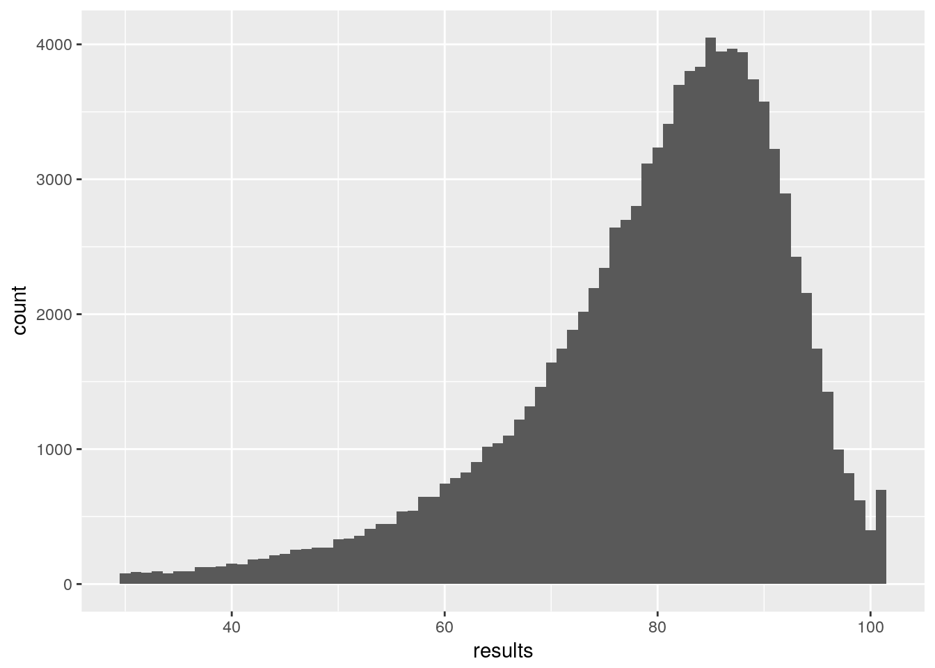
results <-as.vector(MC_results$results$dead)
ggplot()+ aes(results) + geom_density()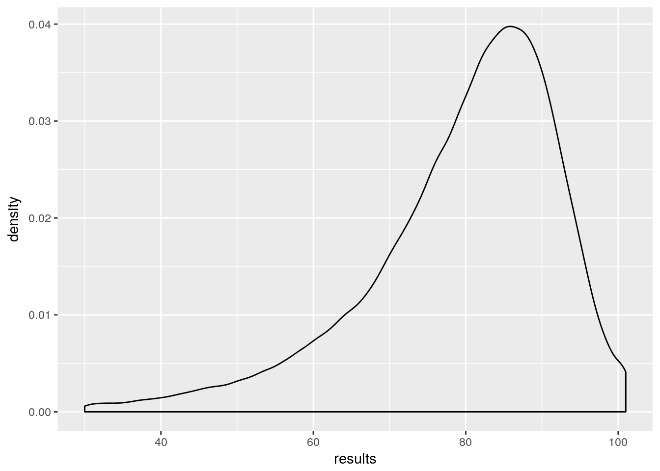
Not using Monte Carlo
So, we have approximately got the distribution of my mortality. However, to properly generalise I need this for ages 0:100 and both males and females. That’s 202 Monte Carlo simulations at about 10 minutes each. Doable, but in doing this I’ve worked out how to calculate the probability without using Monte Carlo. But I want to push this post now, so I’ll make that part 2.
Learning points:
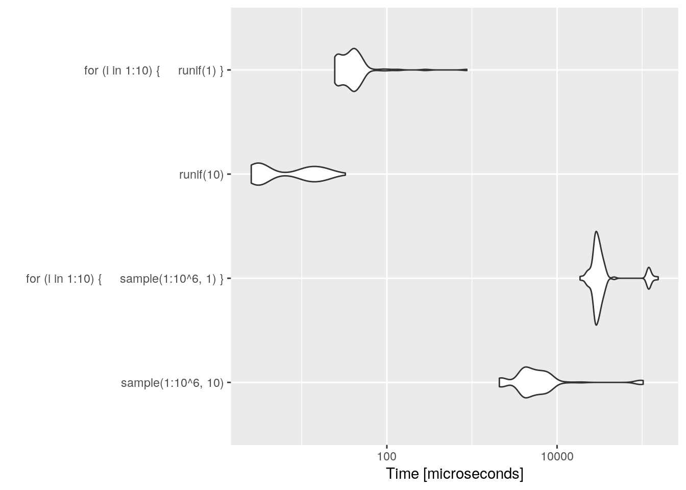
Even if it is more decimal places, R prefers runif to sample(1:10^6).
microbenchmark(sample(1:10^6,10), for(i in 1:10){sample(1:10^6,1)}, runif(10), for(i in 1:10){runif(1)}) %>%
  autoplot