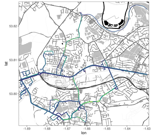
Map of roads that I have cycled, base map in black and white with cycled roads overlaid with viridis coloured palette according to speed cycled.
Map tiles by Stamen Design, under CC BY 3.0. Data by OpenStreetMap, under ODbL.
It has taken a few attempts for me to find cardio that I enjoy, before settling on cycling. I’ve done the first 2 weeks of couch to 5k several times, I dislike running.
But also, I like gamifying my fitness. I wanted to make rude drawings in my GPS trails, inspired by these people, but I can’t see any in the road network near me. So instead I’ve randomly decided that I’m going to visit every (cycleable) road near me.
Most days that I take the bike out I’ll do either my short or longer circuit, or I’ll go to the local-ish Co-Op to grab some groceries. Otherwise I’ll look at the current state of my map and find an area that needs exploring.
Hacking the data together into a map
This is one reason to have a pipeline that ends with all my files in one sensible folder in a sensible-ish format.
While I was trying to work out this problem by hand I found that the {trackeR} library already works with GoldenCheetah format GPS logs, and will map your runs/cycles.
The first problem was that it wanted 1 subplot per session, when I wanted everything on 1 map. The documentation for read_container says that I can read a whole directory, it defaults to 1 session per file, but it will merge different files into 1 session if their timestamps are below a threshold. (e.g. cycle to Co-Op, stop tracking, start tracking <1h later to go home.)
Setting the threshold to Inf worked, and everything became 1 session.
Second problem: some of my cycling logs are not cycling logs, but were weight training with my heart rate monitor. GoldenCheetah’s pipeline ‘helpfully’ logs these as happening at (0,0). Filtering out bad data is always a thing, but in geospatial it looks like we always have to look out for Null Island.
Thirdly, there was a bunch of mess that the plot route function added to my graph that I didn’t want. F2 brings up the source for a function in RStudio, so I copy-pasted the function and removed the bits I didn’t want.
Fourthly, I randomly decided that ‘nearby’ was within a certain bounding box of home. These are arbitary hand-hacked lat/lons that might change with time.
Finally, the function I’m working with will draw a line segment from each point to the next point. This works well when I start and finish at the same place. Sometimes this doesn’t work out. I had a minor crash around the corner of home and stopped tracking, which made the graph have me go in a straight line through some shops and other people’s homes.
The tidy solution would be to throw a NA point at the start or end of each session, before they get merged into 1 session. That doesn’t look simple with this hacky pipeline, so I’ve censored line segments above a certain length. I got the first attempt at getting the right length by box-plotting all lengths and looking at right outliers, but this censored my steep downhill segments! So I went down 1 order of magnitude, and it seems to work.
Using ggplot2 to handle everything in the background is a neat solution. It handles coordinate transformations for breakfast, and I don’t need to filter out duplicate rides along the same road - it just draws a marker over a marker.
I’ve not tweaked the tiles to include cycle-only paths and exclude the national speed limit dual-carriageway that doesn’t exclude bicycles. Technically, legally cycleable, in reality suicidal.
Sidetrack on ‘anonymising’ GPS trails
Obviously it’s not fuly anonymous - road names and lat/lon numbers are still there. GPS is accurate enough to include our driveway in the full graph, so I added a bit more to the lat/lon filters to exclude home and a few more streets. I’m happy with this level of censor, and it’s my data so that’s what counts.
Colour is proportional to speed, but I killed the legend. 1 part because GC turns everything into m/s, 1 part because I’m less interested in the specific colours rather than having some colour that distinguishes cycled roads from uncycled roads.
Code, with some hand-hacked censorship
library(tidyverse)

library(trackeR)

theme_set(ggthemes::theme_few())


file.remove("CENSORED/cycled.png")

# Grab data from GoldenCheetah:

bike = read_directory("CENSORED/activities/",
                      aggregate = TRUE,
                      session_threshold = Inf)

bike[[1]] = bike[[1]][bike[[1]]$latitude!=0,]


# bbox filters
bike[[1]] = bike[[1]][bike[[1]]$longitude  CENSORED,]

bike[[1]] = bike[[1]][bike[[1]]$longitude CENSORED,]# One off to censor home

df <- prepare_route(bike, session = 1, threshold = Inf) %>%
  filter(longitude < 0, latitude > 0) %>%
  mutate(dy = longitude1-longitude0, dx = latitude1-latitude0) %>%
  mutate(dist = sqrt(dy^2 + dx^2)) %>%
  mutate(across(longitude0:latitude1,
                ~ if_else(dist > 1e-3, NA_real_, .x)))
rm(bike) #Bike is a large object, and we're just using df now

plot_everything = function (df, session = 1, zoom = NULL, speed = TRUE, threshold = TRUE,
                            mfrow = NULL, maptype = "toner", messaging = FALSE, ...)
{
session = 1


  centers <- attr(df, "centers")
  ranges_lat <- attr(df, "rangesLat")
  ranges_lon <- attr(df, "rangesLon")
  if (speed) {
    speedRange <- range(df[["speed"]], na.rm = TRUE)
  }
  plotList <- vector("list", length(session))
  names(plotList) <- as.character(session)
  for (ses in session) {
    dfs <- df[df$SessionID == which(ses == session), , drop = FALSE]
    zooms <- if (is.null(zoom))
      centers[centers$SessionID == ses, "zoom"]
    else zoom[which(ses == session)]
    range_lat <- ranges_lat[centers$SessionID == ses, ]
    range_lon <- ranges_lon[centers$SessionID == ses, ]
    map <- ggmap::get_stamenmap(c(left = range_lon$low -
                                    0.001, bottom = range_lat$low - 0.001, right = range_lon$upp +
                                    0.001, top = range_lat$upp + 0.001), zoom = zooms,
                                maptype = maptype, messaging = messaging, ...)
    p <- ggmap::ggmap(map)
    if (speed) {
      p <- p + geom_segment(aes_(x = quote(longitude0),
                                 xend = quote(longitude1), y = quote(latitude0),
                                 yend = quote(latitude1), color = quote(speed)),
                                  data = dfs, lwd = 1, alpha = 0.8, na.rm = TRUE) +
        scale_colour_viridis_c(limits = speedRange, guide = guide_colorbar(title = "Speed"))
    }
    else {
      p <- p + geom_segment(aes_(x = quote(longitude0),
                                 xend = quote(longitude1), y = quote(latitude0),
                                 yend = quote(latitude1)), data = dfs, lwd = 1,
                            alpha = 0.8, na.rm = TRUE)
    }
  }
  p
}

p = plot_everything(df, zoom = 16)+ theme(legend.position = "none")
ggsave("CENSORED/cycled.png", p, width = 29.7, height = 15, units = "cm", dpi = 300)